Unknown Pleasures: pulsars, pop, and plotting

The echoes of history

Sometimes, there are weird connections between very different cultural areas and we see the echoes of history playing out. I'm going to tell you how pulsars, Nobel Prizes, an iconic album cover, Nazi atrocities, and software chart plotting all came to be connected.

The discovery of pulsars

In 1967, Jocelyn Bell was working on her Ph.D. as a post-graduate researcher at the Mullard Radio Astronomy Observatory, near Cambridge in the UK. She had helped build a new radio telescope and now she was operating it. On November 28, 1967, she saw a strikingly unusual and regular signal, which the team nicknamed "little green men". The signal turned out to be a pulsar, a type of star new to science.

This was an outstanding discovery that shook up astronomy. The team published a paper in Nature, but that wasn't the end of it. In 1974, the Nobel committee awarded the Nobel Physics Prize to the team. To everyone on the team except Jocelyn Bell. 

Over the years, there's been a lot of controversy over the decision, with many people thinking she was robbed of her share of the prize, either because she was a Ph.D. student or because she was a woman. Bell herself has been very gracious about the whole thing; she is indeed a very classy lady.

The pulsar and early computer graphics

In the late 1960s, a group of Ph.D. students from Cornell University were analyzing data from the pulsar Bell discovered. Among them was Harold Craft, who used early computer systems to visualize the results. Here's what he said to the Scientific American in 2015: "I found that it was just too confusing. So then, I wrote the program so that I would block out when a hill here was high enough, then the stuff behind it would stay hidden."

Here are three pages from Craft's Ph.D. thesis. Take a close look at the center plot. If Craft had made every line visible, it would have been very difficult to see what was going on. Craft re-imagined the data as if he were looking at it at an angle, for example, as if it were a mountain range ridgeline he was looking down on.  With a mountain ridgeline, the taller peaks hide what's behind them. It was a simple idea, but very effective.

(Credit: JEN CHRISTIANSEN/HAROLD D. CRAFT)

The center plot is very striking. So striking in fact, that it found its way into the Cambridge Encyclopaedia of Astronomy (1977 edition):

(Cambridge Encyclopedia of Astronomy, 1977 edition, via Tim O'Riley)

Joy Division

England in the 1970s was not a happy place, especially in the de-industrialized north. Four young men in Manchester had formed a band and recorded an album. The story goes that one of them, Bernard Sumner, was working in central Manchester and took a break in the city library. He came across the pulsar image in the encyclopedia and liked it a lot.

The band needed an image for their debut album, so they selected this one. They gave it to a recently graduated designer called Peter Saville, with the instructions it was to be a black-on-white image. Saville felt the image would look better white-on-black, so he designed this cover.

This is the iconic Unknown Pleasures album from Joy Division.  

The starkness of the cover, without the band's name or the album's name, set it apart. The album itself was critically acclaimed, but it never rose high in the charts at the time. However, over time, the iconic status of the band and the album cover grew. In 1980, the lead singer, Ian Curtis, committed suicide. The remaining band members formed a new band, New Order, that went on to massive international fame.

By the 21st century, versions of the album cover were on beach towels, shoes, and tattoos.

Joy plots

In 2017, Claus Wilke created a new charting library for R, ggjoy.  His package enabled developers to create plots like the famous Unknown Pleasures album cover. In honor of the album cover, he called these plots joy plots.

Ridgeline plots

This story has a final twist to it. Although joy plots sound great, there's a problem.

Joy Division took their name from a real Nazi atrocity fictionalized in a book called House of Dolls. In some of their concentration camps, the Nazis forced women into prostitution. The camp brothels were called Joy Division. 

The name joy plots was meant to be fun and a callback to an iconic data visualization, but there's little joy in evil. Given this history, Wilke renamed his package ggridges and the plots ridgeline plots. 

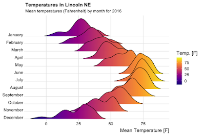
Here's an example of the great visualizations you can produce with it. 

If you search around online, you can find people who've re-created the pulsar image using ggridges.

(Andrew B. Collier via Twitter)

It's not just R programmers who are playing with Unknown Pleasures, Python programmers have got into the act too. Nicolas P. Rougier created a great animation based on the pulsar data set using the venerable Matplotlib plotting package - you can see the animation here.

If you liked this post

You might like these ones:

• Soldiers on the moon: Project Horizon
• Why we have runs on toiler paper
• A masterclass in information visualization: the tube map

Confidence, significance, and p-values

What is truth?

Statistical testing is ultimately all about probabilities and thresholds for believing an effect is there or not. These thresholds and associated ideas are crucial to the decision-making process but are widely misunderstood and misapplied. In this blog post, I'm going to talk about three testing concepts: confidence, significance, and p-values; I'll deal with the hugely important topic of statistical power in a later post.

(peas - not p-values. Author: Malyadri, Source: Wikimedia Commons, License: Creative Commons)

Types of error

To simplify, there are two kinds of errors in statistical testing:

• Type I - false positive. You say there's an effect when there isn't. This is decided by a threshold \(\alpha\), usually set to 5%. \(\alpha\) is called significance.
• Type II - false negative. You say there isn't an effect but there is. This is decided by a threshold \(\beta\) but is usually expressed as the statistical power which is \(1 - \beta\).

In this blog post, I'm going to talk about the first kind of error, Type I.

Distribution and significance

Let's imagine you're running an A/B test on a website and you're measuring conversion on the A branch (\(c_A\)) and on the B branch (\(c_B\)). The null hypothesis is that there's no effect, which we can write as:

\[H_0: c_A - c_B = 0\]

This next piece is a little technical but bear with me. Tests of conversion are usually large tests (mostly, > 10,000 samples in practice). The conversion rate is the mean conversion for all website visitors. Because there are a large number of samples, and we're measuring a mean, the Central Limit Theorem (CLT) applies, which means the mean conversion rates will be normally distributed. By extension from the CLT, the quantity \( c_A - c_B\) will also be normally distributed. If we could take many measurements of \( c_A - c_B\) and the null hypothesis was true, we would theoretically expect the results to look like something like this.

Look closely at the chart. Although I've cut off the x-axis, the values go off to \(\pm \infty\). If all values of \( c_A - c_B\) are possible, how can we reject the null hypothesis and say there's an effect?

Significance - \(\alpha\)

To decide if there's an effect there, we use a threshold. This threshold is referred to as the level of significance and is called \(\alpha\). It's usually set at the 0.05 or 5% level. Confusingly, sometimes people refer to confidence instead, which is 1 - significance, so a 5% significance level corresponds to a 95% confidence level.

In the chart below, I've colored the 95% region around the mean value blue and the 5% region (2.5% at each end) red. The blue region is called the acceptance region and the red region is called the rejection region.

What we do is compare the measurement we actually make with the chart. If our measurement lands in the red zone, we decide there's an effect there (reject the null), if our measurement lands in the blue zone, we'll decide there isn't an effect there (fail to reject the null or 'accept' the null).

One-sided or two-sided tests

On the chart with the blue and the red region, there are two rejection (red) regions. This means we'll reject the null hypothesis if we get a value that's more than a threshold above or below our null value. In most tests, this is what we want; we're trying to detect if there's an effect there or not and the effect can be positive or negative. This is called a two-sided test because we can reject the null in two ways (too negative, too positive).

But sometimes, we only want to detect if the treatment effect is bigger than the control. This is called a one-sided test. Technically, the null hypothesis in this case is:

\[H_0: c_A - c_B \leq 0\]

Graphically, it looks like this:

So we'll reject the null hypothesis only if our measured value lands in the red region on the right. Because there's only one rejection region and it's on one side of the chart, we call this a one-sided test.

p-values

I've very blithely talked about measured values landing in the rejection region or not. In practice, that's not what we do; in practice, we use p-values.

Let's say we measured some value x. What's the probability we would measure this value if the null hypothesis were true (in other words, if there were no effect)? Technically, zero because the distribution is continuous, but that isn't helpful. Let's try a more helpful form of words. Assuming the null hypothesis is true, what's the probability we would see a value of x or a more extreme value? Graphically, this looks something like the green area on the chart below.

Let me say again what the p-value is. If there's no effect at all, it's the probability we would see the result (or a more extreme result) that we measured, or how likely is it that our measurement could have been due to chance alone?

The chart below shows the probability the null hypothesis is true; it shows the acceptance region (blue), the rejection region (red), and the measurement p-value (green). The p-value is in the rejection region, so we'll reject the null hypothesis in this case. If the green overlapped with the blue region, we would accept (fail to reject) the null hypothesis.

Misunderstandings

There are some common misunderstandings around testing that can have quite bad commercial effects.

• 95% confidence is too high a bar - we should drop the threshold to 90%. In effect, this means you'll accept a lot of changes that have no effect. This will reduce the overall effectiveness of your testing program (see this prior blog post for an explanation).
• One-sided tests are OK and give a smaller sample size, so we should use them. This is true, but it's often important to determine if a change is having a negative effect. In general, hypothesis testing tests a single hypothesis, but sadly, people try and read more into test results than they should and want to answer several questions with a single question.
• p-values represent the probability of an effect being present. This is just not true at all.
• A small p-value indicates a big effect. p-values do not make any indication about the size of an effect; a low p-value does not mean there's a big effect.

Practical tensions

In practice, there can be considerable tension between business and technical people over statistical tests. A lot of statistical practices (e.g. 5% significance levels, two-sided testing) are based on experience built up over a long time. Unfortunately, this all sounds very academic to the business person who needs results now and wants to take shortcuts. Sadly, in the long run, shortcuts always catch you up. There's an old saying that's very true: "there ain't no such thing as a free lunch."

Management and technical career tracks: separate but not equal

Promotion paths for technical people

I’ve worked in technology companies and I’ve seen the same question arise several times: what to do with technical people who don’t want to be managers? What do you promote them to?

(Image credit: Louis-Henri de Rudder, source: Old Book Illustrations)

The traditional engineering career ladder emphasizes management as the desired end-goal and devalues anyone not in a management position. Not everyone wants to be a manager and not everyone is good at management. Some people are extremely technically competent and want to stay technical. What are they offered?

Separate, but not equal

Most companies deal with the problem by creating a parallel career path for engineers who don’t want to be managers. This is supposedly separate but equal, but it always ends up being very unequal in the management branch’s favor. The inequality is reflected in job titles. Director is a senior position in most companies and it comes with management responsibility. The equivalent technical role might be ‘Fellow’, which has overtones of putting someone out to grass. A popular alternative is ‘Technical Director’, but note the management equivalent is Director - the engineers get a qualifying word the managers don’t, it’s letting people know the person isn’t a real Director (they're technically a Director, but...). Until you get to VP or C-level, the engineering titles are always worse.

The management and technical tracks have power differences too. The managers get to decide pay raises and promotions and hiring and firing, the technical people don’t. Part of this is obviously why people choose management (and why some people don’t choose management), but often the technical path people aren’t even given a seat at the table. When there are business decisions to be made, the technical people are usually frozen out, even when the business decisions aren't people ones. Sometimes this is legitimate, but most of the time it’s a power thing. The message is clear: if you want the power to change things, you need to be a manager.

A way forward

Here’s what I suggest. The managerial/technical divide is a real one. Not everyone wants to be a manager and there should be a career path upward for them. I suggest having the same job titles for the managerial path and the technical path. There should be no Technical Directors and Directors, just Directors. People on the technical path should be given a seat at the power table and should be equals when it comes to making business decisions. This means managers will have to give up power and it will mean a cultural shift, but if we’re to give meaningful advancement to the engineering track, this is the way it has to be.