Everything you wanted to know about the normal distribution but were afraid to ask

Normal is all around you, and so is not-normal

The normal distribution is the most important statistical distribution. In this blog post, I'm going to talk about its properties, where it occurs, and why it's so very important. I'm also going to talk about how using the normal distribution when you shouldn't can lead to disaster and what you can do about it.

(Ainali, CC BY-SA 3.0 <https://creativecommons.org/licenses/by-sa/3.0>, via Wikimedia Commons)

A rose by any other name

The normal distribution has a number of different names in different disciplines:

• Normal distribution. This is the name used by statisticians and data scientists.
• Gaussian distribution. This is what physicists call it.
• The bell curve. The names used by social scientists and by people who don't understand statistics.

I'm going to call it the normal distribution in this blog post, and I'd advise you to call it this too. Even if you're not a data scientist, using the most appropriate name helps with communication.

What it is and what it looks like

When we're measuring things in the real world, we see different values. For example, if we measure the heights of 10 year old boys in a town, we'd see some tall boys, some short boys, and most boys around the "average" height. We can work out what fraction of boys are a certain height and plot a chart of frequency on the y axis and height on the x axis. This gives us a probability or frequency distribution. There are many, many different types of probability distribution, but the normal distribution is the most important.

(As an aside, you may remember making histograms at school. These are "sort-of" probability distributions. For example, you might have recorded the height of all the children in a class, grouped them into height ranges, counted the number of children in each height range, and plotted the chart. The y axis would have been a count of how many children in that height range. To turn this into a probability distribution, the y axis would become the fraction of all children in that height range. )

Here's what a normal probability distribution looks like. Yes, it's the classic bell curve shape which is exactly symmetrical.

The formula describing the curve is quite complex, but all you need to know for now is that it's described by two numbers: the mean (often written \(\mu\)) and a standard deviation (often written \(\sigma\)). The mean tells you where the peak is and the standard deviation gives you a measure of the width of the curve. 

To greatly summarize: values near the mean are the most likely to occur and the further you go from the mean, the less likely they are. This lines up with our boys' heights example: there aren't many very short or very tall boys and most boys are around the mean height.

Obviously, if you change the mean or the standard deviation, you change the curve, for example, you can change the location of the mean or you can make the curve wider or narrower. It turns out changing the mean and standard deviation just scales the curve because of its underlying mathematical properties. Most distributions don't behave like this; changing parameters can greatly change the entire shape of the distribution (for example, the beta distribution wildly changes shape if you change its parameters). The normal scaling property has some profound consequences, but for now, I'll just focus on one. We can easily map all normal distributions to one standard normal distribution. Because the properties of the standard normal are known, we can easily do math on the standard normal. To put it another way, it greatly speeds up what we need to do.

Why the normal distribution is so important

Here are some normal distribution examples from the real world.

Let's say you're producing precision bolts. You need to supply 1,000 bolts of a precise specification to a customer. Your production process has some variability. How many bolts do you need to manufacture to get 1,000 good ones? If you can describe the variability using a normal distribution (which is the case for many manufacturing processes), you can work out how many you need to produce.

Imagine you're outfitting an army and you're buying boots. You want to buy the minimum number of boots while still fitting everyone. You know that many body dimensions follow the normal distribution (most famously, chest circumference), so you can make a good estimate of how many boots of different sizes to buy.

Finally, let's say you've bought some random stocks. What might the daily change in value be? Under usual conditions, the change in value follows a normal distribution, so you can estimate what your portfolio might be worth tomorrow.

It's not just these three examples, many phenomena in different disciplines are well described by the normal distribution.

The normal distribution is also common because of something called the central limit theorem (CLT). Let's say I'm taking measurement samples from a population, e.g. measuring the speed of cars on a freeway. The CLT says that the distribution of the sample means will follow a normal distribution regardless of the underlying distribution.  In the car speed example, I don't know how the speeds are distributed, but I can calculate a mean and know how certain I am that the mean value is the true (population) mean. This sounds a bit abstract but it has profound consequences in statistics and means that normal distribution comes up time and time again.

Finally, it's important because it's so well-known. The math to describe and use the normal distribution has been known for centuries. It's been written about in hundreds of textbooks in different languages. More importantly, it's very widely taught; almost all numerate degrees will cover it and how to use it. 

Let's summarize why it's important:

• It comes up in nature, in finance, in manufacturing etc.
• It comes up because of the CLT.
• The math to use it is standardized and well-known.

What useful things can I do with the normal distribution?

Let's take an example from the insurance world. Imagine an insurance company insures house contents and cars. Now imagine the claim distribution for cars follows a normal distribution and the claims distribution for house contents also follows a normal distribution. Let's say in a typical year the claims distributions look something like this (cars on the left, houses on the right).

(The two charts look identical except for the numbers on the x and y axis. That's expected. I said before that all normal distributions are just scaled versions of the standard normal. Another way of saying this is, all normal distribution plots look the same.)

What does the distribution look like for cars plus houses?

The long winded answer is to use convolution (or even Monte Carlo). But because the house and car distribution are normal, we can just do:

\(\mu_{combined} = \mu_{houses} + \mu_{cars} \)

\(\sigma_{combined}^2 = \sigma_{houses}^2 + \sigma_{cars}^2\)

So we can calculate the combined distribution in a heartbeat. The combined distribution looks like this (another normal distribution, just with a different mean and standard deviation).

To be clear: this only works because the two distributions were normal.

It's not just adding distributions together. The normal distribution allows for shortcuts if we're multiplying or dividing etc. The normal distribution makes things that would otherwise be hard very fast and very easy.

Some properties of the normal distribution

I'm not going to dig into the math here, but I am going to point out a few things about the distribution you should be aware of.

The "standard normal" distribution goes from \(-\infty\) to \(+\infty\). The further away you get from the mean, the lower the probability, and once you go several standard deviations away, the probability is quite small, but never-the-less, it's still present. Of course, you can't show \(\infty\) on a chart, so most people cut off the x-axis at some convenient point. This might give the misleading impression that there's an upper or lower x-value; there isn't. If your data has upper or lower cut-off values, be very careful modeling it using a normal distribution. In this case, you should investigate other distributions like the truncated normal.

The normal distribution models continuous variables, e.g. variables like speed or height that can have any number of decimal places (but see the my previous paragraph on \(\infty\)). However, it's often used to model discrete variables (e.g. number of sheep, number of runs scored, etc.). In practice, this is mostly OK, but again, I suggest caution.

Abuses of the normal distribution and what you can do

Because it's so widely known and so simple to use, people have used it where they really shouldn't. There's a temptation to assume the normal when you really don't know what the underlying distribution is. That can lead to disaster.

In the financial markets, people have used the normal distribution to predict day-to-day variability. The normal distribution predicts that large changes will occur with very low probability; these are often called "black swan events". However, if the distribution isn't normal, "black swan events" can occur far more frequently than the normal distribution would predict. The reality is, financial market distributions are often not normal. This creates opportunities and risks. The assumption of normality has lead to bankruptcies.

Assuming normality can lead to models making weird or impossible predictions. Let's say I assume the numbers of units sold for a product is normally distributed. Using previous years' sales, I forecast unit sales next year to be 1,000 units with a standard deviation of 500 units. I then create a Monte Carlo model to forecast next years' profits. Can you see what can go wrong here? Monte Carlo modeling uses random numbers. In the sales forecast example, there's a 2.28% chance the model will select a negative sales number which is clearly impossible. Given that Monte Carlo models often use tens of thousands of simulations, it's extremely likely the final calculation will have been affected by impossible numbers.  This kind of mistake is insidious and hard to spot and even experienced analysts make it.

If you're a manager, you need to understand how your team has modeled data. 

• Ask what distributions they've used to model their data. 
• Ask them why they've used that distribution and what evidence they have that the data really is distributed that way. 
• Ask them how they're going to check their assumptions. 
• Most importantly, ask them if they have any detection mechanism in place to check for deviation from their expected distribution.

History - where the normal came from

Rather unsatisfactorily, there's no clear "Eureka!" moment for the discovery of the distribution, it seems to have been the accumulation of the work of a number of mathematicians. Abraham de Moivre  kicked off the process in 1733 but didn't formalize the distribution, leaving Gauss to explicitly describe it in 1801 [https://medium.com/@will.a.sundstrom/the-origins-of-the-normal-distribution-f64e1575de29].

Gauss used the normal distribution to model measurement errors and so predict the path of the asteroid Ceres [https://en.wikipedia.org/wiki/Normal_distribution#History]. This sounds a bit esoteric, but there's a point here that's still relevant. Any measurement taking process involves some form of error. Assuming no systemic bias, these errors are well-modeled by the normal distribution. So any unbiased measurement taking today (e.g opinion polling, measurements of particle mass, measurement of precision bolts, etc.) uses the normal distribution to calculate uncertainty.

In 1810, Laplace placed the normal distribution at the center of statistics by formulating the Central Limit Theorem. 

The math

The probability distribution function is given by:

\[f(x) = \frac{1}{\sigma \sqrt{2 \pi}} e ^ {-\frac{1}{2} ( \frac{x - \mu}{\sigma}) ^ 2  }\]

\(\sigma\) is the standard deviation and \(\mu\) is the mean. In the normal distribution, the mean is the same as the mode is the same as the median.

This formula is almost impossible to work with directly, but you don't need to. There are extensive libraries that will do all the calculations for you.

Adding normally distributed parameters is easy:

\(\mu_{combined} = \mu_{houses} + \mu_{cars} \)

\(\sigma_{combined}^2 = \sigma_{houses}^2 + \sigma_{cars}^2\)

Wikipedia has an article on how to combine normally distributed quantities, e.g. addition, multiplication etc. see  https://en.wikipedia.org/wiki/Propagation_of_uncertainty.

Is this coin biased?

Tossing and turning

A few months ago, someone commented on one of my blog posts and asked how you work out if a coin is biased or not. I've been thinking about the problem since then. It's not a difficult one, but it does bring up some core notions in probability theory and statistics which are very relevant to understanding how A/B testing works, or indeed any kind of statistical test. I'm going to talk you through how you figure out if a coin is biased, including an explanation of some of the basic ideas of statistical tests.

The trial

A single coin toss is an example of something called a Bernoulli trial, which is any kind of binary decision you can express as a success or failure (e.g. heads or tails). For some reason, most probability texts refer to heads as a success. 

We can work out what the probability is of getting different numbers of heads from a number of tosses, or more formally, what's the probability \(P(k)\) of getting \(k\) heads from \(n\) tosses, where \(0 < k ≤ n\)? By hand, we can do it for a few tosses (three in this case):

Number of heads (k)	Combinations (n)	Count	Probability
0	TTT	1	1/8
1	HTT  THT  TTH	3	3/8
2	THH  HTH  HHT	3	3/8
4	HHH	1	1/8

But what about 1,000 or 1,000,000 tosses - we can't do this many by hand, so what can we do? As you might expect, there's a formula you can use: 

\[P(k) = \frac{n!} {k!(n-k)!} p^k (1-p)^{n-k}\]

\(p\) is the probability of success in any trial, for example, getting a head. For an unbiased coin \(p=0.5\); for a coin that's biased 70% heads \(p=0.7\). 

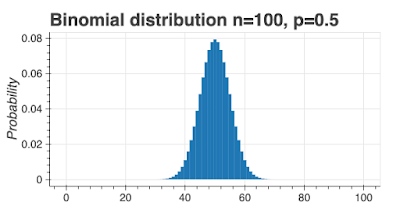
If we plot this function for an unbiased coin (\(p=0.5\)), where \(n=100\), and \(0 < k ≤ n\), we see this probability distribution:

This is called a binomial distribution and it looks a lot like the normal distribution for large (\(> 30\)) values of \(n\). 

I'm going to re-label the x-axis as a score equal to the fraction of heads: 0 means all tails, 0.5 means \(\frac{1}{2}\) heads, and 1 means all heads. With this slight change, we can more easily compare the shape of the distribution for different values of \(n\). 

I've created two charts below for an unbiased coin (\(p=0.5\)), one with \(n=20\) and one with \(n=40\). Obviously, the \(n=40\) chart is narrower, which is easier to see using the score as the x-axis. 

As an illustration of what these charts mean, I've colored all scores 0.7 and higher as red. You can see the red area is bigger for \(n=20\) than \(n=40\). Bear in mind, the red area represents the probability of a score of 0.7 or higher. In other words, if you toss a fair coin 20 times, you have a 0.058 chance of seeing a score of 0.7 or more, but if you toss a fair coin 40 times, the probability of seeing a 0.7 score drops to 0.008.

These charts tell us something useful: as we increase the number of tosses, the curve gets narrower, meaning the probability of getting results further away from \(0.5\) gets smaller. If we saw a score of 0.7 for 20 tosses, we might not be able to say the coin was biased, but if we got a score of 0.7 after 40 tosses, we know this score is very unlikely so the coin is more likely to be biased.

Thresholds

Let me re-state some facts:

• For any coin (biased or unbiased) any score from 0 to 1 is possible for any number of tosses.
• Some results are less likely than others; e.g. for an unbiased coin and 40 tosses, there's only a 0.008 chance of seeing a score of 0.7.

We can use probability thresholds to decide between biased and non-biased coins.  We're going to use a threshold (mostly called confidence) of 95% to decide if the coin is biased or not. In the chart below, the red areas represent 5% probability, and the blue areas 95% probability.

Here's the idea to work out if the coin is biased. Set a confidence value, usually at 0.05. Throw the coin \(n\) times, record the number of heads and work out a score. Draw the theoretical probability chart for the number of throws (like the one I've drawn above) and color in 95% of the probabilities blue and 5% red. If the experimental score lands in the red zones, we'll consider the coin to be biased, if it lands in the blue zone, we'll consider it unbiased.

This is probabilistic decision-making. Using a confidence of 0.05 means we'll wrongly say a coin is biased 5% of the time. Can we make the threshold higher, could we use 0.01 for instance? Yes, we could, but the cost is increasing the number of trials.

As you might expect, there are shortcuts and we don't actually have to draw out the chart. In Python, you can use the binom_test function in the stats package. 

To simplify, binom_test has three arguments:

• x - the number of successes

• n - the number of samples

• p - the hypothesized probability of success

It returns a p-value which we can use to make a decision.

Let's see how this works with a confidence of 0.05. Let's take the case where we have 200 coin tosses and 140 (70%) of them come up heads. We're hypothesizing that the coin is fair, so \(p=0.5\).

from scipy import stats

print(stats.binom_test(x=140, n=200, p=0.5))

the p-value we get is 1.5070615573524992e-08 which is way less than our confidence threshold of 0.05 (we're in the red area of the chart above). We would then reject the idea the coin is fair.

What if we got 112 heads instead?

from scipy import stats

print(stats.binom_test(x=115, n=200, p=0.5))

This time, the p-value is 0.10363903843786755, which is greater than our confidence threshold of 0.05 (we're in the blue area of the chart), so the result is consistent with a fair coin (we fail to reject the null).

What if my results are not significant? How many tosses?

Let's imagine you have reason to believe the coin is biased. You throw it 200 times and you see 115 heads. binom_test tells you you can't conclude the coin is biased. So what do you do next?

The answer is simple, toss the coin more times.

The formulae for the sample size, \(n\), is:

\[n = \frac{p(1-p)} {\sigma^2}\]

where \(\sigma\) is the standard error. 

Here's how this works in practice. Let's assume we think our coin is just a little biased, to 0.55, and we want the standard error to be \(\pm 0.04\). Here's how many tosses we would need: 154. What if we want more certainty, say \(\pm 0.005\), then the number of tosses goes up to 9,900. In general, the bigger the bias, the fewer tosses we need, and the more certainty we want the more tosses we need. 

If I think my coin is biased, what's my best estimate of the bias?

Let's imagine I toss the coin 1,000 times and see 550 heads. binom_test tells me the result is significant and it's likely my coin is biased, but what's my estimate of the bias? This is simple, it's actually just the mean, so 0.55. Using the statistics of proportions, I can actually put a 95% confidence interval around my estimate of the bias of the coin. Through math I won't show here, using the data we have, I can estimate the coin is biased 0.55 ± 0.03.

Is my coin biased?

This is a nice theoretical discussion, but how might you go about deciding if a coin is biased? Here's a step-by-step process.

1. Decide on the level of certainty you want in your results. 95% is a good measure.
2. Decide the minimum level of bias you want to detect. If the coin should return heads 50% of the time, what level of bias can you live with? If it's biased to 60%, is this OK? What about biased to 55% or 50.5%?
3. Calculate the number of tosses you need.
4. Toss your coin.
5. Use binom_test to figure out if the coin deviates significantly from 0.5.

Other posts like this

• What's a probability distribution?
• The null hypothesis test

What's a probability distribution?

Why should you care about probability distributions?

Using the wrong probability distribution can be extremely expensive for businesses:

• for businesses using machinery (factories, vehicles, aircraft, etc.), it can lead to parts being changed too frequently or too infrequently
• for businesses relying on returning customers, it can lead to substantial under or over-estimates of revenue and/or targeting the wrong customers with promotions
• for businesses forecasting future sales by territory and/or product, it can lead to poor territory allocation or poor product resource allocation.

Given that it's so important, what is a probability distribution, and what are some examples?

What's a probability distribution?

At its simplest, a probability distribution tells you how likely an outcome is given some input. For example, how is sales probability distributed by price, or how likely is a component to fail in the next month? 

If something is certain to occur, the probability is 1, if it's certain not to occur, the probability is zero.  Let's imagine a component lasts a maximum of 6 months before failure. Our probability distribution might show the probability of failure on days 1 to 180. The sum of all failure probabilities for all days must sum to 1.

In the real world, data is noisy and we don't expect real data to exactly follow theoretical distributions, but given enough data, the match should be close enough for us to reason about what's going on.

Uniform distribution - gambling and manufacturing

If the probability is the same for all input values, the distribution is uniform.

Let's imagine we're manufacturing candy, and we want to have equal numbers of red, blue, green, black, and white sweets in a packet. In theory, here's what we should observe.

But in reality, there's random noise so we might see something like this below. We can quantify the difference between the expected distribution and the actual distribution, which tells us something about the variability in the manufacturing process. 

The uniform distribution also occurs in gambling, for example, lotteries or dice games.

Reading more

Uniform distribution description by NIST

Binomial distribution - pass/fail and conversion

Each customer who comes into a store or who visits a website will either buy or not buy, which we can turn into a conversion rate. We can model these kinds of pass/fail processes using the binomial distribution. Here's the probability distribution.

The binomial distribution shows us the probability of measuring different results given an underlying 'truth'. Let's imagine the 'true' conversion rate was 0.04, we might not measure 0.04 due to sampling error, instead, we might measure 0.045 or 0.055, depending on how many samples we take. It's important to understand what this means: 

• There is uncertainty in our measurement. 
• The smaller the sample, the bigger the uncertainty.

Although many technical people understand this, most non-technical people do not, which can lead to tension.

Reading more

Yale stats

Poisson distribution - waiting in line

Imagine you're a bank serving customers with ATMs at a location. ATMs are expensive, but you don't want to keep people waiting in long lines to do their transactions, it's bad for business. So how do you balance the cost of an ATM against its use? By modeling how many people are using the ATM over a time period.

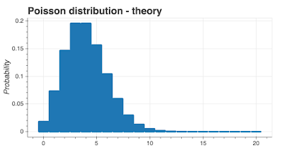
It turns out, the number of people who visit an ATM over a time period can be modeled using the Poisson distribution, which I've shown below. This gives us a way of assessing how much variation there might be in usage and therefore how many machines we might want to install. 

The Poisson distribution is often used to model counting processes. It's very attractive because it has an unusual feature, the standard deviation for the distribution is \(\sqrt{\gamma}\) where \(\gamma\) is the mean. Unfortunately, this property makes it a little too attractive; it's sometimes used when it shouldn't be.

Reading more

The Poisson Distribution and Poisson Process Explained

Exponential distribution

How long does a car battery last? How long do phone calls last? When will the next earthquake occur? These durations typically follow the exponential distribution (which is strongly related to the Poisson distribution). I've shown this distribution below.

Reading more

The exponential distribution

Power law distribution - finding fraud

How are incomes distributed in a population? How might you find fraud in the pattern of digits in expenses? It turns out, the distribution of the first digits in invoices follows a power-law distribution. The chart below shows a generic power-law distribution - for fraud detection, it's 'flipped'.

Reading more

Power law distribution

Normal distribution - almost everywhere, but not quite

What's the probability distribution for male soldiers' chest measurements? How are the results of A/B tests distributed? What about the distribution of measurement errors? All these, and many, many more follow the normal distribution, which is also called the Gaussian distribution or the bell curve. If you only learn one distribution, this is the one to learn. 

The properties of this distribution are extremely well-known, and every student of statistics and probability theory will know them. It's ubiquitous because of something called the Central Limit Theorem, which, simplifying a great deal, says that the sum of samples from any distribution follows a normal distribution.

Because it's everywhere, for some people, it's the only distribution they know. Like the old saying goes, if you only have a hammer, every problem is a nail. This distribution can be over-used, with bad consequences.

Here's the distribution. It ought to look familiar.

Reading more

The normal distribution

Lognormal distribution

How long do visitors spend on web pages? What about the distribution of internet traffic? Or the distribution of city sizes? These all follow a log-normal distribution that looks like the example below. The lognormal distribution is quite common in business.

Note the 'fat tail' or 'long tail' on the right-hand side. Many businesses have been caught out because they assumed sales or market risk followed a normal distribution when in fact they followed a lognormal distribution.

There's a variation of the Central Limit Theorem that yields log-normal distributions instead of normal distributions.

Reading more

Limpert, Eckhard, Werner A. Stahel, and Markus Abbt. "Log-normal distributions across the sciences: keys and clues" BioScience 51.5 (2001): 341-352.

Other distributions

There are lots and lots of different distributions. I saw a list of 90 the other day. Almost all of them are esoteric and apply in a very limited set of cases. You don't have to know all of them but you should be aware that choosing the right distribution is important to make the correct estimates. The distributions I've listed in this blog post are probably the most important, and you should know them and their properties.

As you asked nicely, here is a list of some distributions.

Alpha Distribution

Anglit Distribution

Arcsine Distribution

Beta Distribution

Beta Prime Distribution

Bradford Distribution

Burr Distribution

Burr12 Distribution

Cauchy Distribution

Chi Distribution

Chi-squared Distribution

Cosine Distribution

Double Gamma Distribution

Double Weibull Distribution

Erlang Distribution

Exponential Distribution

Exponentiated Weibull Distribution

Exponential Power Distribution

Fatigue Life (Birnbaum-Saunders) Distribution

Fisk (Log Logistic) Distribution

Folded Cauchy Distribution

Folded Normal Distribution

Fratio (or F) Distribution

Gamma Distribution

Generalized Logistic Distribution

Generalized Pareto Distribution

Generalized Exponential Distribution

Generalized Extreme Value Distribution

Generalized Gamma Distribution

Generalized Half-Logistic Distribution

Generalized Inverse Gaussian Distribution

Generalized Normal Distribution

Gilbrat Distribution

Gompertz (Truncated Gumbel) Distribution

Gumbel (LogWeibull, Fisher-Tippetts, Type I Extreme Value) Distribution

Gumbel Left-skewed (for minimum order statistic) Distribution

HalfCauchy Distribution

HalfNormal Distribution

Half-Logistic Distribution

Hyperbolic Secant Distribution

Gauss Hypergeometric Distribution

Inverted Gamma Distribution

Inverse Normal (Inverse Gaussian) Distribution

Inverted Weibull Distribution

Johnson SB Distribution

Johnson SU Distribution

KSone Distribution

KStwo Distribution

KStwobign Distribution

Laplace (Double Exponential, Bilateral Exponential) Distribution

Left-skewed Lévy Distribution

Lévy Distribution

Logistic (Sech-squared) Distribution

Log Double Exponential (Log-Laplace) Distribution

Log Gamma Distribution

Log Normal (Cobb-Douglass) Distribution

Log-Uniform Distribution

Maxwell Distribution

Mielke’s Beta-Kappa Distribution

Nakagami Distribution

Noncentral chi-squared Distribution

Noncentral F Distribution

Noncentral t Distribution

Normal Distribution

Normal Inverse Gaussian Distribution

Pareto Distribution

Pareto Second Kind (Lomax) Distribution

Power Log Normal Distribution

Power Normal Distribution

Power-function Distribution

R-distribution Distribution

Rayleigh Distribution

Rice Distribution

Reciprocal Inverse Gaussian Distribution

Semicircular Distribution

Student t Distribution

Trapezoidal Distribution

Triangular Distribution

Truncated Exponential Distribution

Truncated Normal Distribution

Tukey-Lambda Distribution

Uniform Distribution

Von Mises Distribution

Wald Distribution

Weibull Maximum Extreme Value Distribution

Weibull Minimum Extreme Value Distribution

Wrapped Cauchy Distribution

Continuous or discrete - shaken or stirred?

Some quantities are discrete and some are continuous. A discrete quantity is something like a sales territory (e.g. Germany, Ireland, Spain) or customer count (you can't have 0.5 of a customer). A continuous quantity can take any value, for example, speed can be 45.2 kph, 120.01 kph, and so on. Some distributions apply to both continuous and discrete, and some apply only to continuous or discrete. To muddy the waters, sometimes continuous distributions are used to approximately model discrete quantities.

Business examples

Vehicles

Imagine you're running a delivery vehicle fleet. You need to keep your vehicles on the road, but you need to keep an eye on maintenance costs. You decide to use math to guide your decisions, so you work out the average lifetime for different components. You have two components A and B with the same lifetimes in miles. If either component fails, you have to tow the vehicle, which is very expensive.

• Component A. Lifetime is 150,000 miles.
• Component B. Lifetime is 150,000 miles.

A vehicle comes in for maintenance with 149,000 miles on the odometer. Should you replace components A and B?

As you might expect, there's a gotcha. Without knowing the probability distribution for failures, we can't make these decisions. For example, a windshield might have a uniform failure rate distribution, with the probability of failure for miles 1-100 the same as the probability of failure for miles 100,000-100,100. A clutch may have a failure rate that increases with mileage, the probability of failure at miles 100,000-100,100 being much higher than the probability of failure at miles 0-100. Because we know what a clutch and a windshield are, we might decide to replace the clutch and leave the windshield. But what if A and B were a serpentine belt and a heat shield?

The only way to make rational decisions is to understand what distribution the probability of failure follows, which may well be very different for different components (e.g. car seats vs. tires).

Marketing

A new analyst is studying the market for luxury goods in Germany. They have partial data for the fraction of the population that have a certain income. Using what they have, they assume their data is normally distributed and they make a forecast for the fraction of the population that will have an income high enough to afford luxury items. Do you think their forecast will be too low, just right, or too high?

Incomes are usually log-normally distributed, so the analyst, in this case, has chosen the wrong distribution. Because the lognormal has a very long right tail, the analyst's estimate is likely to be an underestimate and may be substantially out. A competitor might not make the same mistake.

Takeaways

I've interviewed people who claim data science on their resumes, but only know the normal distribution. If you assume your data is normal, when in reality it's log-normal or Poisson, things are going to go badly wrong for you. Any analyst in business needs to be very comfortable with different distributions and needs to know which may be applicable and when.

How to (maybe) win at dice

Does God play dice with the universe?

Imagine I gave you an ordinary die, not special in any way, and I asked you to throw the die and record your results (how many 1s, how many 2s, etc.). What would you expect the results to be? Do you think you could win by choosing some numbers rather than others? Are you sure?

(Image source: Wikimedia Commons. Author: Diacritica. License: Creative Commons.)

What you might expect

Let's say you thew the die 12,000 times, you might expect a probability distribution something like this. This is a uniform distribution where all results are equally likely.

You know you'll never get an absolutely perfect distribution, so in reality, your results might look something like this for 12,000 throws. 

The deviations from the expected values are random noise that we can quantify. Further, we know that by adding more dice throws, random noise gets less and less and we approach the ideal uniform distribution more closely. 

I've simulated dice throws in the plots below, the top chart is 12,000 throws and the chart on the bottom is 120,000 throws. The blue bars represent the actual results, the black circle represents the expected value, and the black line is the 95% confidence interval. Note how the results for 120,000 throws are closer to the ideal than the results from 12,000 throws.

What happened in reality - not what you expect

My results are simulations, but what happens when you throw dice thousands of times in the real world?

There's a short history of probability theorists and statisticians throwing dice and recording the results.

• Weldon threw 12 dice 26,306 times by hand and sent the results to his friend Francis Galton.
• Iversen ran an experiment where 219 dice were rolled 20,000 times.

Weldon's data set is widely used to illustrate statistical concepts, especially after Pearson used it to explain his \(\chi^2\) technique in 1900. 

Despite the excitement you see at the craps tables in Las Vegas, throwing dice thousands of times is dull and is, therefore, an ideal job for a computer. In 2009, Zachariah Labby created apparatus for throwing dice and recording the scores using a camera and image processing. You can read more about his apparatus and experimental setup here. He 'threw' 12 dice 26,306 times and his machine recorded the results. 

In the chart below, the blue bars are his results, the black circle is the expected result, and the black line is the 95% confidence interval. I've taken the results from all 12 dice, so my throw count is \(12 \times 26,306\).

This doesn't look like a uniform distribution. To state the obvious, 1 and 6 occurred more frequently than theory would suggest - the deviation from the uniform distribution is statistically significant. The dice he used were not special dice, they were off-the-shelf standard unbiased dice. What's going on?

Unbiased dice are biased

Take a very close look at a normal die, the type pictured at the start of this post which is the kind of die you buy in shops.

By convention, opposite faces on dice sum to 7, so 1 is opposite 6, 3 is opposite to 4, and so on. Now look very closely again at the picture at the start of the post. Look at the dots on the face of the dice. Notice how they're indented. Each hole is the same size, but obviously, the number of holes on each face is different. Let's think of this in terms of weight. Imagine we could weigh each face of the dice. Let's pair up the faces, each side is paired with the face opposite it. Now let's weigh the faces and compare them.

The greatest imbalance in weights is the 1-6 combination. This imbalance is what's causing the bias.

Obviously, the bias is small, but if you roll the die enough times, even a small bias becomes obvious. 

Vegas here I come - or not...

So we know for dice bought in shops that 1 and 6 are ever so slightly more likely to occur than theory suggests. Now you know this, why aren't you booking your flight to Las Vegas? You could spend a week at the craps tables and make a little money.

Not so fast.

Let's look at the dice they use in Vegas.

(Image source: Wikimedia Commons. Author: Alper Atmaca License: Creative Commons.)

Notice that the dots are not indented. They're filled with colored material that's the same density as the rest of the dice. In other words, there's no imbalance, Vegas dice will give a uniform distribution, and 1 and 6 will occur as often as 2, 3, 4, or 5. You're going to have to keep punching the clock.

Some theory

Things are going to get mathematical from here on in. There won't be any new stories about dice or Vegas.

How did I get the expected count and error bars for each dice score? Let's say I threw the dice \(x\) times, it seems obvious we would get an expected count of \(\frac{x}{6}\) for each score, but why? What about the standard error?

Let's re-think the dice as a Bernoulli trial. Let's choose a score, say 1. If we throw the dice and it shows a 1, we consider that a success. If it shows anything else, we consider it a failure. Because we have a Bernoulli trial, we can use the binomial distribution to model the results.

Using Wikipedia's notation:

• \(n\) is the number of throws
• \(p\) is the probability of getting a 1, which is \(\frac{1}{6}\)
• \(q = 1- p\) is the probability of getting 2-6, which is \(\frac{5}{6}\)

So, again using Wikipedia's handy summary, for \(n\) throws:

• The mean is \(np = 12 \times 26,306 \times \frac{1}{6} = 52,612\)
• The standard deviation is \(\sqrt{npq} = \sqrt{12 \times 26,306 \times \frac{1}{6} \times \frac{5}{6}} = 209.388\) 
• The 95% confidence interval is \(52,202 \) to \(53,022\) (standard deviation by 1.96).

Publications

Academics live or die by publications and by citations of their publications. Labby's work has rightly been widely cited on the internet. I keep hoping that some academic will be inspired by Labby and use modern robotic technology and image recognition to do huge (million-plus) classical experiments, like tossing coins or selecting balls from an urn. It seems like an easy win to be widely cited!