What's a violin plot and how to make one?

What's a violin plot?

Over the last few years, violin plots and their derivatives have become a lot more common; they're a 'sort of' smoothed histogram. In this blog post, I'm going to explain what they are and why you might use them.

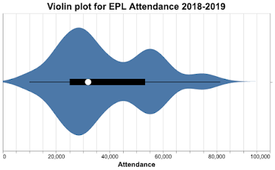
To give you an idea of what they look like, here's a violin plot of attendance at English Premier League (EPL) matches during the 2018-2019 season. The width of the plot indicates the relative proportion of matches with that attendance; we can see attendance peaks around 27,000, 55,000, and 75,000, but no matches had zero attendance. 

Violin plots get their name because they sort of resemble a violin (you'll have to allow some creative license here).

As we'll see, violin plots avoid the problems of box and whisker plots and the problems of histograms. The cost is greatly increased computation time, but for a modern computer system, violin plots are calculated and plotted in the blink of an eye. Despite their advantages, the computational cost is why these plots have only recently become popular.

Summary statistics - the mean etc.

We can use summary statistics to give a numerical summary of the data. The most obvious statistics are the mean and standard deviation, which are 38,181 and 16,709 respectively for the EPL 2018 attendance data. But the mean can be distorted by outliers and the standard deviation implies a symmetrical distribution. These statistics don't give us any insight into how attendance was distributed.

The median is a better measure of central tendency in the presence of outliers, and quartiles work fine for asymmetric distributions. For this data, the median is 31,948 and the upper and lower quartiles are 25,034 and 53,283. Note the median is a good deal lower than the mean and the upper and lower quartiles are not evenly spaced, suggesting a skewed distribution. The quartiles give us an indication of how skewed the data is.

So we should be just fine with median and quartiles - or are there problems with these numbers too?

Box and whisker plots

Box and whisker plots were introduced by Tukey in the early 1970s and evolved since then, currently, there are several slight variations. Here's a box and whisker plot for the EPL data for four seasons in the most common format; the median, upper and lower quartiles, and the lowest and highest values are all indicated. We have a nice visual representation of our distribution.

The box and whisker plot encodes a lot of data and strongly indicates if the distribution is skewed. Surely this is good enough?

The problem with boxplots

Unfortunately, box and whisker plots can hide important features of the data. This article from Autodesk Research gives a great example of the problems. I've copied one of their key figures here.

("Same Stats, Different Graphs: Generating Datasets with Varied Appearance and Identical Statistics through Simulated Annealing", Justin Matejka, George Fitzmaurice, ACM SIGCHI Conference on Human Factors in Computing Systems, 2017)

The animation shows the problem nicely; different distributions can give the same box and whisker plots. This doesn't matter most of the time, but when it does matter, it can matter a lot, and of course, the problem is hidden.

Histograms and distributions

If boxplots don't work, what about histograms? Surely they won't suffer from the same problem? It's true they don't, but they suffer from another problem; bin count, meaning the number of bins.

Let's look at the EPL data again, this time as a histogram.

Here's the histogram with a bin count of 9.

Here it is with a bin count of 37.

And finally, with a bin count of 80.

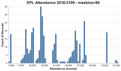
Which of these bin counts is better? The answer is, it depends on what you want to show. In some cases, you want a large number of bins, in other cases, a small number of bins. As you can appreciate, this isn't helpful, especially if you're at the start of your career and you don't have a lot of experience to call on. Even later in your career, it's not helpful when you need to move quickly.

An evolution of the standard histogram is using unequal bin sizes. Under some circumstances, this gives a better representation of the distribution, but it adds another layer of complexity; what should the bin sizes be? The answer again is, it depends on what you want to do and your experience.

Can we do better?

Enter the violin plot

The violin plot does away with bin counts by using probability density instead. It's a plot of the probability density function (pdf) that could have given rise to the measured data. 

In a handful of cases, we could estimate the pdf using parametric means when the underlying data follows a well-known distribution. Unfortunately, in most real-world cases, we don't know what distribution the data follows, so we have to use a non-parametric method, the most popular being kernel density estimation (kde). This is almost always done using a Gaussian estimator, though other estimators are possible (in my experience, the Gaussian calculation gives the best result anyway, but see this discussion on StackOverflow). The key parameter is the bandwidth, though most kde algorithms attempt to size their bandwidth automatically. From the kde, the probability density is calculated (a trivial calculation).

Here's the violin plot for the EPL 2018 data.

It turns out, violin plots don't have the problems of box plots as you can see from this animation from Autodesk Research. The raw data changes, the box plot doesn't, but the violin plot changes dramatically. This is because all of the data is represented in the violin plot.

("Same Stats, Different Graphs: Generating Datasets with Varied Appearance and Identical Statistics through Simulated Annealing", Justin Matejka, George Fitzmaurice, ACM SIGCHI Conference on Human Factors in Computing Systems, 2017)

Variations on a theme, types of violin plot, ridgeline plots, and mirror density plots

The original form of the violin plot included median and quartile data and you often see violin plots presented like this - a kind of hybrid of violin and box and whisker. This is how the Seaborn plotting package draws Violin plots (though this chart isn't a Seaborn visualization).

Now, let's say we want to compare the EPL attendance data over several years. One way of doing it is to show violin plots next to each other, like this.

Another way is to show two plots back-to-back, like this. This presentation is often called a mirror density plot.

We can show the results from multiple seasons with another form of violin plot called the ridgeline plot. In this form of plot, the charts are deliberately overlapped, letting you compare the shape of the distributions better. They're called ridgeline plots because they sort of look like a mountain ridgeline.

This plot shows the most obvious feature of the data, the 2019-2020 season was very different from the seasons that went before; a substantial number of matches were held with zero attendees.

When should you use violin plots?

If you need to summarize a distribution and represent all of the data, a violin plot is a good choice. Depending on what you're trying to do, it may be a better choice than a histogram and it's always a better choice than box and whisker plots.

Aesthetically, a violin plot or one of its variations is very appealing. You shouldn't underestimate the importance of clear communication and visual appeal. If you think your results are important, surely you should present them in the best way possible - and that may well be a violin plot.

Reading more

"Statistical computing and graphics, violin plots: a box plot-density trace synergism", Jerry Hintze, Ray Nelson, American Statistical Association, 1998. This paper from Hintze and Nelson is one of the earlier papers to describe violin plots and how they're defined, it goes into some detail on the process for creating them. 

"Violin plots explained" is a great blog post that provides a nice explanation of how violin plots work.

"Violin Plots 101: Visualizing Distribution and Probability Density" is another good blog post proving some explanation on how to build violin plots.

Mouse jiggling: the good, the bad, and the ugly

What's a mouse jiggler?

Recently, I was reading Hacker News and one of the contributors mentioned a mouse jiggler. I'd never heard of one before, so I searched around. I was both horrified and fascinated by what I discovered.

A mouse jiggler is a device that randomly 'jiggles' your mouse so it appears that you're at your computer. It prevents the screen saver from kicking in and it keeps your status as active in Slack and Zoom. Here's a picture of one type of mouse jiggler.

(Jamsim1975, CC BY-SA 4.0, via Wikimedia Commons)

The good

As it turns out, mouse jigglers are used by law enforcement during raids. One of the agents is tasked with getting to the suspect's computer quickly and setting up the mouse jiggler. The goal is to stop the computer from locking up; if that happens the suspect has to provide their password or a court has to order them to do so. Far better to stop the computer from locking up in the first place.

In the old days, the FBI and other agencies used software mouse jigglers; the mouse motion was set by software installed on a USB stick. Mechanical mouse jigglers are better because they don't rely on the availability of USB ports and they don't rely on security settings on the suspect's computer (not all systems will allow software to be installed via USB).

This blog post has some interesting things to say about mouse jigglers and other software/hardware used during raids.

The bad

There's a reason why security teams have computers lock themselves after a few minutes of user inactivity and the reason is security. Leaving a computer unattended and unlocked is bad, leaving a computer unattended and unlocked with a mouse jiggler over extended periods is even worse. If I were a CISO, I would ban mouse jigglers - or better still, make sure that no one feels the need to use one.

The ugly

For everyone who's not law enforcement, why would you want a jiggler? The sad answer seems to be fooling employee surveillance software. Instead of trusting their employees or measuring by results, some companies have installed surveillance software that tracks mouse usage (mouse use = work). Jigglers are an attempt to circumvent these kinds of trackers.

Jigglers have been around for a while and now there's software to detect them; you too can detect if your employees are jiggling. In response, some of the newer jigglers offer random and subtle jiggles that are harder to detect. I can see a jiggling arms race coming.

The reviews for this jiggler on Amazon are enlightening; there are 2,612 of them, an astonishing number, and the product has a 5-star rating overall. Many of the reviews mention fooling IT surveillance software. If you don't like this one, there are plenty of other models to choose from, many with over 1,000 reviews. 

Think about what this says. There are enough people who're concerned about surveillance to spawn a mini-industry for $30 devices. These devices add no value - it's not like a mouse or a keyboard or a camera. As one of the reviewers said, the jiggler lets them go to the bathroom without feeling like it's being noted. It's all about trust, or the lack of it.

If people are using mouse jigglers at your company, it's an indication that something has gone quite wrong.

Ice ice baby

Is this the coolest/most Canadian data set ever?

Late last year, I was studying for a machine learning course and I was looking for a data set I could use for the course capstone project. I settled on English Premier League data, but not before I had a serious look at what's probably the coolest (and most Canadian) dataset I've ever seen.

(cogdogblog, CC BY 2.0, via Wikimedia Commons)

The icicle atlas

The University of Toronto Physics Department has a large dataset on icicles created as part of a research project to understand the factors important for icicle formation, size, and shape. Under laboratory conditions, they grew 237 icicles, capturing movies and images of their growth. 

As part of the growth process, they varied speed, salinity, and water source, obviously having a little fun with their choice of water sources as you'll see in the atlas. As it turns out, the ridges that sometimes form in icicles are due to impurities in the water (maybe all of us need impurities to be interesting😉).

All the images, movies, and data are covered by a creative commons license. You can see all their icicle data on their icicle atlas page - the related links at the bottom of the page are fantastic.

Icicle pictures

You can view the rogues' gallery of icicle pictures here. Here are some pictures of my favorite icicles from the gallery.

(University of Toronto Physics Department, Icicle Atlas, Creative Commons License.)

Icicle movies

You can see videos of how most of the icicles formed. It's kind of interesting and restful to watch - the opposite of watching a fire burning, but still hypnotic and engaging. Here's a video that I found restful.

(University of Toronto Phyics Department, Icicle Atlas, Creative Commons License.)

If you want more, there's a YouTube channel of the movies from the atlas.

Ice Ice baby

This winter, I'm going to see icicles form on my gutters. I've seen some weird formations over the years, and now I know that temperature, wind, and water purity govern the size and shape of icicles. It's nice to know that we can still take time to understand the processes that form the world around us.

Even though I better understand how icicles form, I know they can damage my gutters and house. Pretty as they are, I'm still going to smash them away.

Football crazy: predicting Premier League football match results

I can get a qualification and be rich!

A long time ago, I was part of a gambling syndicate. A friend of mine had some software that predicted the results of English football (soccer) matches and at the time, betting companies offered fixed-price odds for certain types of bets. My friend noticed his software predicted 3-2 away wins more often than the betting company's odds would suggest. Over the course of a season, we had a 20% return on our gambling investment. 

(Ronnie Macdonald from Chelmsford, United Kingdom, CC BY 2.0, via Wikimedia Commons)

During the COVID lockdown, I took the opportunity to learn R and did a long course that included a capstone project. I decided to see if I could forecast English Premier League (EPL) matches. If I succeeded, I could get a qualification and get rich too! What's not to like? Here's the story of what I did and what happened.

Premier League data

There's an eighteenth-century recipe for a hare dish that supposedly includes the instructions "First, catch your hare." The first step in any project like this is getting your data.

(Robert Scoble from Half Moon Bay, USA, CC BY 2.0, via Wikimedia Commons)

I got match results going back to the start of the league (1993) from football-data. The early data is only match results, but later data includes red cards and some other measurements.

TransferMarkt has data on transfer fees, foreign-born players, and team age, but the data's only available from 2011.

At the time of the project, I couldn't find any other free data sources. There were and are paid-for sources, but they were way beyond what I was willing to pay.

I knew going into the next phase of the project that this wasn't a very big data set with not that many fields. As it turned out, data was a severely limiting factor.

What factors are important?

I had a set of initial hypotheses for factors that might be important for final match scores, here are most of them:

• team cost - more expensive teams should win more games
• team age - younger teams perform better
• prior points - teams with more points win against teams with fewer points
• foreign-born players - the more non-English players on the team, the more the team will win
• previous match results - successful (winning) teams win more matches
• home-field advantage
• disciplinary record - red and yellow card history might be an indicator of risk-taking
• season effects - as the season wears on, teams take more risks to win matches

I found evidence that most of these did in fact have an impact.

Here's strong evidence of home-field advantage. Note how it goes away during the 2020-2021 season when matches were played without fans.

Here's goal difference vs. team cost difference. The more expensive team tends to win.

Here's goal difference vs. mean prior goal difference. Teams that scored more goals before tend to score more goals in their current match.

I found more relationships you can read about if you're interested.

Machine learning

Thinking back to my gambling syndicate, I decided to forecast the score of each match rather than just win/lose/draw. My loss function was the RMSE of the goal difference between the predicted score and the actual score. To avoid COVID oddities, I removed the 2020-2021 season (the price being a smaller data set). Of course, I used a training and holdout dataset and cross-validation. 

The obvious question is, which model machine learning models work? I decided to try a whole bunch of them:

• Naive mean score model. A simple model that’s just the mean scores of the (training) data set.
• Generalized Linear Model. A form of ordinary linear regression.
• Glmnet. Fits lasso and elastic-net regularized generalized linear models.
• SVM. Support Vector Machines - boundary-based regression. After some experimentation, I selected the svmRadial form of SVM, which uses a non-linear kernel function.
• KNN. K-nearest neighbors. Given that EPL scores are all in close proximity to one another, we might expect this model to return good results.
• Neural nets.
• XGB Linear. This is linear modeling with extreme gradient boosting. Extreme gradient boosting has gathered a lot of attention over the last few years and may be one of the most used machine learning models today.
• XGB Tree. This is a decision tree model with extreme gradient boosting.
• Random Forest.

The model results weren't great. For the KNN model, here's how the RMSE for full-time away goals varied with n.

Note the RMSE scale - the lowest it goes to is 1.1 goals and it's plain that adding more n will only take us a little closer to 1.1. Bear in mind, football is a low-scoring game, and being off by 1 goal is a big miss.

It was the same story for random forest.

In fact, it was the same story for all of the models. Here are my final results. My model forecast home goals and away goals.

The naive means model is the simplest and all my sophisticated models could do is give me a few percentage points improvement.

Improving the results

Perhaps the most obvious way forward is combining models to improve RMSE. I'm reluctant to do that until I can get better individual model results. There's a philosophical issue at play; for me, the ensemble approach feels a bit "spray and pray".

In my view, data shortage is the main problem:

• My data set was only in the low thousands of matches. 
• Some teams join the Premier League for just a season and then get relegated - I don't model their history prior to joining the league. 
• I removed the COVID season of 2020-2021. 
• I only had team value and disciplinary data for ten or so seasons. 
• Of course, I only modeled the Premier League.

Football is a low-scoring game, famous for its upsets. It may well be that it's just too random underneath to make useful predictions at the individual match level. 

What's next?

I wasn't able to predict EPL results with any great accuracy, but I submitted my report and got my grade. If you want to read my report, you can read it here.

At the end of the 2021 season, I saw some papers published on the COVID effect on match results. I had similar results months before. Perhaps I should have submitted a paper myself.

At some point, I might revive this project if I can get new data. I still occasionally hunt for new data sources, but sadly, I haven't found any. My dreams of retiring to a yacht on the Mediterranean will have to wait.

Why conditional probability screwiness matters for business

Things are not what they seem

Many business decisions come down to common sense or relatively simple math. But applying common sense to conditional probability problems can lead to very wrong results as we'll see. As data science becomes more and more important for business, decisions involving conditional probability will arise more often. In this blog post, I'm going to talk through some counter-intuitive conditional probability examples and where I can, I'll tell you how they arise in a business context.

(These two pieces of track are the same size. Ag2gaeh, CC BY-SA 4.0, via Wikimedia Commons.)

Testing for diseases

This is the problem with the clearest links to business. I'll explain the classical form of the problem and show you how it can come up in a business context.

Imagine there's some disease affecting a small fraction of the population, say 1%. A university develops a great test for the disease:

• If you have the disease, the test will give you a positive result 99% of the time. 
• If you don't have the disease, the test will give you a negative result 99% of the time.

You take the test and it comes back positive. What's the probability you have the disease? 

(COVID test kit. Centers for Disease Control and Prevention, Public domain, via Wikimedia Commons)

The answer is 50%.

If you want an explanation of the 50% number, read the section "The math", if you want to know how it comes up in business, skip to the section "How it comes up in business".

The math

What's driving the result is the low prevalence of the disease (1%). 99% of the people who take the test will be uninfected and it's this that pushes down the probability of having the disease if you test positive. 

There are at least two ways of analyzing this problem, one is using a tree diagram and one is using Bayes' Theorem. In a previous blog post, I went through the math in detail, so I'll just summarize the simpler explanation using a tree diagram. To make it easier to understand, I'll assume a population of 10,000.

Of the 10,000 people, 100 have the disease, and 9,900 do not. Of the 100, 99 will test positive for the disease. Of the 9,900, 99 will test positive for the disease. In total 99 + 99 will test positive, of which only 99 will have the disease. So 50% of those who test positive will have the disease.

How it comes up in business

Instead of disease tests, let's think of websites and algorithms. Imagine you're the CEO of a web-based business. 1% of the visitors to your website become customers. You want to identify who'll become a customer, so you task your data science team with developing an algorithm based on users' web behavior. You tell them the test is to distinguish customers from non-customers.

They come back with a complex test for customers that's 99% true for existing customers and 99% false for non-customers. Do you have a test that can predict who will become a customer and who won't?

This is the same problem as before, if the test is positive for a user, there's only a 50% chance they'll become a customer.

How many daughters?

This is a classic problem and shows the importance of describing a problem exactly. Exactly, in this case, means using very very precise English.

Here's the problem in its original form from Martin Gardner:

1. Mr. Jones has two children. The older child is a girl. What is the probability that both children are girls?
2. Mr. Smith has two children. At least one of them is a boy. What is the probability that both children are boys?

(What's the probability of two girls? Circle of Robert Peake the elder, Public domain, via Wikimedia Commons)

The solution to the first problem is simple. Assuming boys or girls are equally likely, then it's 50%.

The second problem isn't simple and has generated a great deal of debate, even 60 years after Martin Gardner published the puzzle. Depending on how you read the question, the answer is either 50% or 33%. Here's Khovanova's explanation:

"(i) Pick all the families with two children, one of which is a boy. If Mr. Smith is chosen randomly from this list, then the answer is 1/3.

(ii) Pick a random family with two children; suppose the father is Mr. Smith. Then if the family has two boys, Mr. Smith says, “At least one of them is a boy.” If he has two girls, he says, “At least one of them is a girl.” If he has a boy and a girl he flips a coin to say one or another of those two sentences. In this case, the probability that both children are the same sex is 1/2."

In fact, there are several other possible interpretations.

What does this mean for business? Some things that sound simple aren't and differences in the precise way a problem is formulated can give wildly different answers.

Airline seating

Here's the problem stated from an MIT handout:

"There are 100 passengers about to board a plane with 100 seats. Each passenger is assigned a distinct seat on the plane. The first passenger who boards has forgotten his seat number and sits in a randomly selected seat on the plane. Each passenger who boards after him either sits in his or her assigned seat if it is empty or sits in a randomly selected seat from the unoccupied seats. What is the probability that the last passenger to board the plane sits in her assigned seat?"

You can imagine a lot of seat confusion, so it seems natural to assume that the probability of the final passenger sitting in her assigned seat is tiny. 

(Ken Iwelumo (GFDL 1.2, GFDL 1.2 or GFDL 1.2), via Wikimedia Commons)

Actually, the probability of her sitting in her assigned seat is 50%.

StackOverflow has a long discussion on the solution to the problem that I won't repeat here.

What does this mean for business? It's yet another example of our intuition letting us down.

The Monty Hall problem 

This is the most famous of all conditional probability problems and I've written about it before. Here's the problem as posed by Vos Savant:

"A quiz show host shows a contestant three doors. Behind two of them is a goat and behind one of them is a car. The goal is to win the car.

The host asked the contestant to choose a door, but not open it.

Once the contestant has chosen a door, the host opens one of the other doors and shows the contestant a goat. The contestant now knows that there’s a goat behind that door, but he or she doesn’t know which of the other two doors the car’s behind.

Here’s the key question: the host asks the contestant "do you want to change doors?".

Once the contestant decided whether to switch or not, the host opens the contestant's chosen door and the contestant wins the car or a goat.

Should the contestant change doors when asked by the host? Why?"

(The original uploader was Kuxu at French Wikipedia., CC BY-SA 3.0, via Wikimedia Commons)

Here are the results.

• If the contestant sticks with their initial choice, they have a ⅓ chance of winning.
• If the contestant changes doors, they have a ⅔ chance of winning.

I go through the math in these two previous blog posts "The Monty Hall Problem" and "Am I diseased? An introduction to Bayes theorem".

Once again, this shows how counter-intuitive probability questions can be.

What should your takeaway be, what can you do?

Probability is a complex area and common sense can lead you wildly astray. Even problems that sound simple can be very hard. Things are made worse by ambiguity; what seems a reasonable problem description in English might actually be open to several possible interpretations which give very different answers.

(Sound judgment is needed when dealing with probability. You need to think like a judge, but you don't have to dress like one. InfoGibraltar, CC BY 2.0, via Wikimedia Commons)

If you do have a background in probability theory, it doesn't hurt to remind yourself occasionally of its weirder aspects. Recreational puzzles like the daughters' problem are a good refresher.

If you don't have a background in probability theory, you need to realize you're liable to make errors of judgment with potentially serious business consequences. It's important to listen to technical advice. If you don't understand the advice, you have three choices: get other advisors, get someone who can translate, or hand the decision to someone who does understand.