What's a violin plot?
Over the last few years, violin plots and their derivatives have become a lot more common; they're a 'sort of' smoothed histogram. In this blog post, I'm going to explain what they are and why you might use them.
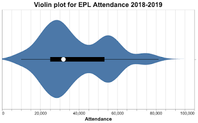
To give you an idea of what they look like, here's a violin plot of attendance at English Premier League (EPL) matches during the 2018-2019 season. The width of the plot indicates the relative proportion of matches with that attendance; we can see attendance peaks around 27,000, 55,000, and 75,000, but no matches had zero attendance.
Violin plots get their name because they sort of resemble a violin (you'll have to allow some creative license here).
As we'll see, violin plots avoid the problems of box and whisker plots and the problems of histograms. The cost is greatly increased computation time, but for a modern computer system, violin plots are calculated and plotted in the blink of an eye. Despite their advantages, the computational cost is why these plots have only recently become popular.
Summary statistics - the mean etc.
We can use summary statistics to give a numerical summary of the data. The most obvious statistics are the mean and standard deviation, which are 38,181 and 16,709 respectively for the EPL 2018 attendance data. But the mean can be distorted by outliers and the standard deviation implies a symmetrical distribution. These statistics don't give us any insight into how attendance was distributed.
The median is a better measure of central tendency in the presence of outliers, and quartiles work fine for asymmetric distributions. For this data, the median is 31,948 and the upper and lower quartiles are 25,034 and 53,283. Note the median is a good deal lower than the mean and the upper and lower quartiles are not evenly spaced, suggesting a skewed distribution. The quartiles give us an indication of how skewed the data is.
So we should be just fine with median and quartiles - or are there problems with these numbers too?
Box and whisker plots
Box and whisker plots were introduced by Tukey in the early 1970s and evolved since then, currently, there are several slight variations. Here's a box and whisker plot for the EPL data for four seasons in the most common format; the median, upper and lower quartiles, and the lowest and highest values are all indicated. We have a nice visual representation of our distribution.
The box and whisker plot encodes a lot of data and strongly indicates if the distribution is skewed. Surely this is good enough?
The problem with boxplots
Unfortunately, box and whisker plots can hide important features of the data. This article from Autodesk Research gives a great example of the problems. I've copied one of their key figures here.
The animation shows the problem nicely; different distributions can give the same box and whisker plots. This doesn't matter most of the time, but when it does matter, it can matter a lot, and of course, the problem is hidden.
Histograms and distributions
If boxplots don't work, what about histograms? Surely they won't suffer from the same problem? It's true they don't, but they suffer from another problem; bin count, meaning the number of bins.
Let's look at the EPL data again, this time as a histogram.
Here's the histogram with a bin count of 9.
Here it is with a bin count of 37.
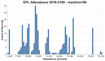
And finally, with a bin count of 80.
Which of these bin counts is better? The answer is, it depends on what you want to show. In some cases, you want a large number of bins, in other cases, a small number of bins. As you can appreciate, this isn't helpful, especially if you're at the start of your career and you don't have a lot of experience to call on. Even later in your career, it's not helpful when you need to move quickly.
An evolution of the standard histogram is using unequal bin sizes. Under some circumstances, this gives a better representation of the distribution, but it adds another layer of complexity; what should the bin sizes be? The answer again is, it depends on what you want to do and your experience.
Can we do better?
Enter the violin plot
The violin plot does away with bin counts by using probability density instead. It's a plot of the probability density function (pdf) that could have given rise to the measured data.
In a handful of cases, we could estimate the pdf using parametric means when the underlying data follows a well-known distribution. Unfortunately, in most real-world cases, we don't know what distribution the data follows, so we have to use a non-parametric method, the most popular being kernel density estimation (kde). This is almost always done using a Gaussian estimator, though other estimators are possible (in my experience, the Gaussian calculation gives the best result anyway, but see this discussion on StackOverflow). The key parameter is the bandwidth, though most kde algorithms attempt to size their bandwidth automatically. From the kde, the probability density is calculated (a trivial calculation).
Here's the violin plot for the EPL 2018 data.
It turns out, violin plots don't have the problems of box plots as you can see from this animation from Autodesk Research. The raw data changes, the box plot doesn't, but the violin plot changes dramatically. This is because all of the data is represented in the violin plot.
Variations on a theme, types of violin plot, ridgeline plots, and mirror density plots
The original form of the violin plot included median and quartile data and you often see violin plots presented like this - a kind of hybrid of violin and box and whisker. This is how the Seaborn plotting package draws Violin plots (though this chart isn't a Seaborn visualization).
Now, let's say we want to compare the EPL attendance data over several years. One way of doing it is to show violin plots next to each other, like this.
Another way is to show two plots back-to-back, like this. This presentation is often called a mirror density plot.
We can show the results from multiple seasons with another form of violin plot called the ridgeline plot. In this form of plot, the charts are deliberately overlapped, letting you compare the shape of the distributions better. They're called ridgeline plots because they sort of look like a mountain ridgeline.
This plot shows the most obvious feature of the data, the 2019-2020 season was very different from the seasons that went before; a substantial number of matches were held with zero attendees.
When should you use violin plots?
If you need to summarize a distribution and represent all of the data, a violin plot is a good choice. Depending on what you're trying to do, it may be a better choice than a histogram and it's always a better choice than box and whisker plots.
Aesthetically, a violin plot or one of its variations is very appealing. You shouldn't underestimate the importance of clear communication and visual appeal. If you think your results are important, surely you should present them in the best way possible - and that may well be a violin plot.
Reading more
"Statistical computing and graphics, violin plots: a box plot-density trace synergism", Jerry Hintze, Ray Nelson, American Statistical Association, 1998. This paper from Hintze and Nelson is one of the earlier papers to describe violin plots and how they're defined, it goes into some detail on the process for creating them.
"Violin plots explained" is a great blog post that provides a nice explanation of how violin plots work.
"Violin Plots 101: Visualizing Distribution and Probability Density" is another good blog post proving some explanation on how to build violin plots.


No comments:
Post a Comment